The Dual Axis
A dive into the interplay between sparsity and dimensionality
Introduction
Plato, in search of a way to define what comprises a human being, arrived at the conclusion that a person is ‘a featherless biped’. Diogenes, a contemporary (and a philosopher worth studying in his own right), brought a plucked chicken to Plato’s Academy and proclaimed ‘Here is Plato’s man’. In response, Plato added ‘with flat, broad nails’ to correct for the mistake. I love this story not just for Diogenes’s facetious response but also because of how it illustrates a fundamental epistemological problem: what comprises an object? If we choose to describe an object by a series of characteristics, how many do we need before we can be confident with what object we are describing? In the above example, the characteristics of ‘bipedal’ and ‘featherless’ were insufficient, and ‘flat and broad nails’ were added for further clarity.
If we were to describe humans as belonging to a matrix of different animal characteristics, according to Plato, we would need at least three to differentiate a human from other animals. It could be said that the intrinsic dimension of a person is therefore 3. Intrinsic dimensionality is the number of variables needed to minimally represent a dataset. It is deeply related to the manifold hypothesis, which states that for many high-dimensional datasets such as audio, vision, and language, their data-generating process actually lies on a low-dimensional manifold. This poses an interesting question: from what manifold are neural networks generated?
Orthogonal to the question of dimensionality is the question of sparsity. It is a common myth that humans only use 10% of their brain, an absurd claim given that the brain roughly consumes 20% of your body’s overall calories. In reality, we are often using the whole of our brain; however, there does appear to be evidence to suggest that not all neurons are fired. Rather, there appears to be sparseness in which neurons are fired for any given stimulus.
It turns out this is true for neural networks as well. While modern compute infrastructure is optimized for dense computation, it’s likely that over 90% of such computations are unnecessary. This is a major problem, especially as the demand for gigantic foundation models captures the public’s zeitgeist. Some estimates put yearly power consumption at 80+ terawatt-hours globally! While it currently accounts for roughly 1% of global power consumption (far from the human 20%), it is still a cause for concern given the shifting climate. Therefore it is a noble goal to pursue more energy efficient (read minimal) computations to achieve strong results.
Therefore, as we aim to achieve higher levels of artificial intelligence, we must ask ourselves what is the nature of intelligence. More specifically, we pose the question of “What minimally constitutes intelligence?” This can be posed both in the context of the number of dimensions we require to represent intelligence and how many operations are necessary to perform intelligent tasks.
Background
I thought I’d tackle the background of this blog a little differently than before. As some of you may know, I have been accepted as a graduate student at the University of Alberta. My goals are to perform research on the nature of neural network training, specifically focusing on large language models. As you might expect, I will have to read a great many number of papers! In preparation for that, I will be presenting the background for this blog as paper reviews. This works out as the bulk of the work for this blog involves paper reproduction. The works that I aim to reproduce are mainly related to the nature of neural networks.
Measuring the Intrinsic Dimension of Objective Landscapes
The paper that spawned the paper with a thousand citations investigates the impact of low-rank training for a variety of different tasks and neural architectures. Given a parameter set of size \(n\), the authors employ a random projection \(\theta^{n} = \theta^{n}_{0} + P\theta^{m}\) where \(\theta^{n}\) represents the parameters of a network, \(\theta^{n}_{0}\) represents the initial parameters of a network, \(P^{n \times m}\) is a random projection matrix, and \(\theta^{m}\) represents a lower-dimensional set of trainable parameters. Cleverly, the authors initialize \(\theta^{m}\) to 0, meaning they take advantage of the original model initialization (a trick employed by many of the modern parameter-efficient fine-tuning methods we use today). They show that it is possible to achieve 90% of a fully parameterized model’s task accuracy with an incredibly compressed parameter space. Furthermore, their experiments suggest that architecture (fully connected vs convolutional networks) and task difficulty (MNIST vs Shuffled MNIST) have significant impacts on compressibility. To me, it provides a great argument for the inductive bias of a neural network architecture. Furthermore, if the data-generating process is embedded in a low-dimensional manifold, then it is only natural that neural networks themselves would fall into the manifold hypothesis as well.
Intrinsic Dimensionality Explains the Effectiveness of Language Model Fine-Tuning
The paper that actually spawned the paper with a thousand citations explores the intrinsic dimensionality of fine-tuning from a set of pre-trained weights. Specifically, they tune a RoBERTa model following a similar methodology to Li et al. Distinctly, they augment the random projections of Li et al.’s previous work to \(\theta^{n}_{i} = \theta^{n}_{0, i} + \lambda_{i}P\theta^{d-m}_{i}\) where they add a trainable parameter \(\lambda_i\) for the \(i\)-th layer, and \(m\) is the number of layers. This is to allow the algorithm (called Structurally Aware Intrinsic Dimension or SAID) to dampen layers that are unneeded in the fine-tuning. To enable the size of \(P\), they perform a Fast Food transform instead of a dense random projection. Once again, they found that the intrinsic dimension was tied to the difficulty of the fine-tuning task. This served as a direct inspiration for the intuition behind the development of Low-Rank Adaptation (LORA)
The Lottery Ticket Hypothesis: Finding Sparse, Trainable neural Networks
In this work, the authors propose the Lottery Ticket hypothesis. This hypothesis states that there exists a subnetwork within an over-parameterized dense model that, when initialized and trained, can match the accuracy of the original model. They then go further and propose a conjecture that states that SGD seeks to find these subnetworks and trains them. In support of their argument, they found that they may iteratively prune a network by first training a model, pruning the model, then resetting the subnetwork to its initial weights, which may then be trained to equal or greater accuracy in equal or fewer training iterations. They call this methodology of training, pruning, and resetting Iterative Magnitude Pruning (IMP). Interestingly, they show that while a pruned network may be reinitialized and trained from scratch, this fails at a certain level of sparsity, and the weight initialization does have an impact on the performance of the retraining. While they experiment on both a feed-forward and convolutional neural network, they do so on different datasets. I would be curious to see how the model architecture affects the sparsity rates that may be achieved. They did, however, experiment with pruning only the feed-forward or convolution weights. However, as the feed-forward weights vastly outnumber the convolutional weights, I feel as though this is not an apt comparison (they were able to achieve better performance on pruning the convolutional layers, see appendix H.6).
Deconstructing Lottery Tickets: Zeros, Signs, and the Supermask
In this work, the authors explore the dynamics of the lottery ticket through several different experiments. First, they begin by defining several different Mask Criteria to derive a suitable mask for a neural network. They then found the following:
- Initialization is not critical to the performance of iterative pruning. Although still lower in accuracy than keeping the initial weights, keeping the sign is sufficient for providing good results.
- Masking out weights (Hadamard product with 0) greatly improves performance over simply freezing the initial weight. This is interesting because it supports the idea that the weight being masked was already being shifted towards zero in the initial stages of optimization.
- They show the existence of supermasks, masks that when applied to an untrained set of weights provide greatly improved performance over random chance. Notably, this supermask is still derived from the training process.
While the work is interesting, I found it rather unsurprising. Beginning with the first point, it appears natural that the initial sign is important as it most defines the differences in angle. The second point appears to be clear as well; masking can be thought of as taking a gradient step equal to the original weight size. Certainly, a few weights were set to be zero. Finally, given that the supermask was derived from the training process, at a minimum, it would be equivalent to performing gradient descent for the 0 terms.
The Dual Axis
So, why do we care? Well, you can think of dimensionality and sparsity as representing the intrinsic number of parameters necessary to complete a task. There has been quite a large body of work that explores either dimensionality or sparsity. Interestingly, both have deep motivations stemming from the drive to discover more efficient and faster algorithms. As I alluded to earlier, the investigations into dimensionality have exploded with the advent of large language models. Their ability to generalize to new, unseen tasks with little (in the context of fine-tuning) to no (in the case of zero-shot prompting) additional training is extraordinary in the field of deep learning. Therefore, a rich ecosystem has arisen in discovering new parameter-efficient fine-tuning methods that leverage the lower dimensionality of solving tasks.
In contrast, network pruning has a more storied history, with investigations dating back to 1989 with Le Cun’s investigation into optimal brain damage.
Combined, they define two very different but related ideas: what are the minimal number of parameters necessary to perform a task? Here, I would like to introduce the dual axis of dimension and sparsity. Dimension addresses the question of ‘What is the minimum set of attributes do I need to describe a concept?’ Sparsity, however, addresses the problem of ‘How many numbers do I need in order to determine the attributes?’ Let’s try to uncover some of the interplay between these two axes.
Initial MNIST Model
To begin, we must define an initial model for which we will attempt to compress. Below is a simplified convolutional neural network that is loosely inspired by the LeNet5 architecture. For those of you who’ve read my previous work, you will recognize this model. What I would distinctly like to draw attention to is the difference in activation function for this model: I am now using ReLU. The reason for this is because for the intrinsic dimensionality, we must propagate backwards through a massive projection matrix \(P\). Therefore, I chose to use ReLU to improve gradient flow and numerical stability.
class MnistExampleNet(nn.Module):
  """
  A simple convolutional network inspired by LeNet5 for MNIST classification

  Parameters:
      c (int): Number of channels in the first convolutional layer.
  """
  def __init__(self, c: int=32):
    super(MnistExampleNet, self).__init__()
    self.conv1 = nn.Conv2d(1, c, kernel_size=5, bias=False)
    self.pool = nn.MaxPool2d(kernel_size=2, stride=2)
    self.conv2 = nn.Conv2d(c, c * 2, kernel_size=5, bias=False)
    self.fc1 = nn.Linear(c * 2 * 4 * 4, 10, bias=False)

  def forward(self, x):
    x = self.pool(F.relu(self.conv1(x)))
    x = self.pool(F.relu(self.conv2(x)))
    x = x.flatten(1)
    x = self.fc1(x)
    return x
Methodology
I now introduce our experimental methodology. First, I initialize and store an initial model. This model will serve as the initial parameter set shared across all of our experiments. I set the baseline model as this initial model and train it for 10 epochs normally to classify MNIST images. Following this, I evaluate three distinct training paradigms using the initial model’s parameters prior to training:
- Training using Intrinsic Dimensionality (ID)
- Training using Iterative Magnitude Pruning (IMP)
- Training using both Intrinsic Dimensionality and Iterative Magnitude Pruning (ID + IMP)
For each methodology, we train for 10 epochs, with IMP and ID IMP having 4 pruning rounds. To my knowledge, this is the first work that aims to combine both intrinsic dimensionality training with iterative magnitude pruning. Below is the code for the third methodology. To implement this behavior, we use the newly ported torch.func.functional_call. This enables us to easily decouple the functional form of a module from its weights, which are managed by the state dictionary and saved as an attribute. Understanding this code will give you a good understanding of how I implemented the first two methodologies.
class FunctionalPrunedInstrinsicWrapper(nn.Module):
    def __init__(self, module, intrinsic_dimension, prune_ratio):
        """
        Wrapper to estimate the intrinsic dimensionality of the
        objective landscape for a specific task given a specific model
        :param module: pytorch nn.Module
        :param intrinsic_dimension: dimensionality within which we search for solution
        """
        super(FunctionalPrunedInstrinsicWrapper, self).__init__()
        theta = nn.Parameter(torch.zeros((intrinsic_dimension, )))
        self.module = module
        self.prune_ratio = prune_ratio
        self.register_parameter("theta", theta)

        for name, param in module.named_parameters():
            name = name.replace('.', '-')
            if param.requires_grad:
              param.requires_grad=False
              initial_weight = param.clone().detach().requires_grad_(False)
              matrix_size = initial_weight.size() + (intrinsic_dimension, )
              projection = (
                    torch.randn(matrix_size, requires_grad=False)
                    / intrinsic_dimension ** 0.5
                )
              self.register_buffer(f'initial_{name}', initial_weight)
              self.register_buffer(f'mask_{name}', torch.ones(initial_weight.size()))
              self.register_buffer(f'projection_{name}', projection)

    def forward(self, x):
        state_dict = {}
        for name, _ in self.module.named_parameters():
            n = name.replace('.', '-')
            V = torch.matmul(getattr(self, f'projection_{n}'), self.theta)
            param = getattr(self, f'initial_{n}') + torch.squeeze(V, -1)
            state_dict[name] = param * getattr(self, f'mask_{n}')
        x = functional_call(self.module, state_dict, x)
        return x

    def prune_and_reinitialize(self, n_round):
        nn.init.zeros_(self.theta)
        for name, param in self.module.named_parameters():
            n = name.replace('.', '-')
            V = torch.matmul(getattr(self, f'projection_{n}'), self.theta)
            X = getattr(self, f'initial_{n}') + torch.squeeze(V, -1)
            num_prune_params = int((1-self.prune_ratio**n_round) * X.nelement())
            mask = getattr(self, f'mask_{n}')
            topk = torch.topk(torch.abs(X).view(-1), k=num_prune_params, largest=False)
            mask.view(-1)[topk.indices] = 0
            setattr(self, f'mask_{n}', mask)
Results
Overall Comparison
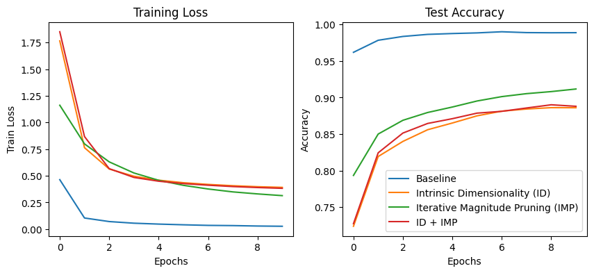
For evaluations of methodologies 1 and 2, we aim to use the same 90% metric as was introduced in the original intrinsic dimensionality paper. Given that our initial model, once trained, hovers around 98.5% accuracy, we aim for our first two methodologies to achieve around 88.65% accuracy. For the third methodology we aim to find a lottery ticket network whereby the model performs roughly equivalent to the intial model (in this case the ID model) with the maximum amount of pruning prior to performance degradation. Below, we compare the training loss and the test accuracy across our different training methodologies. Recall that all methodologies share a set of initial weights despite traversing the optimization differently (due to the stochastic ordering of the minibatches). We note that all three training methodologies hover around the same performance and are far worse than the original baseline model. Notably, despite only having access to 256 parameters, Intrinsic Dimensionality performs favorably overall.

Comparison of Different Pruning Rounds for IMP
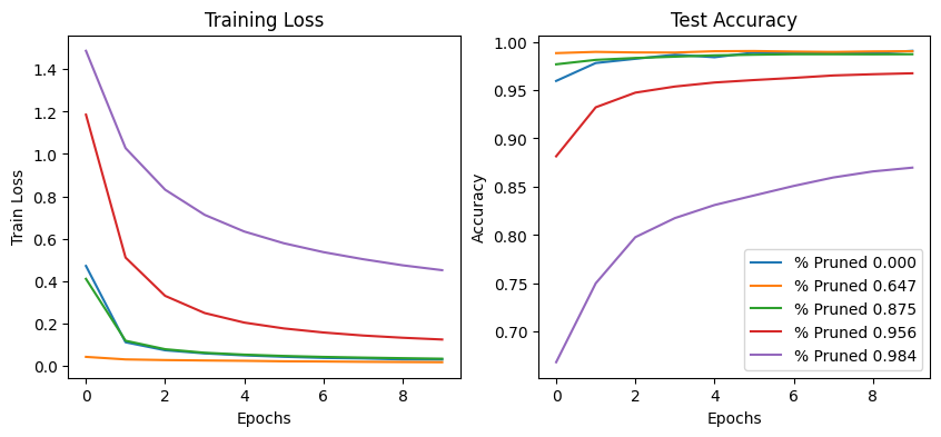
Following our initial assessment, we explore the varying loss curves for Iterative Magnitude Pruning. Shown below are the loss curves for the iterative magnitude pruning training methodology, with greater sparsity denoting a later pruning round. We note that, much like the findings of Zhou et al.

Comparison of Different Pruning Rounds for IMP + ID
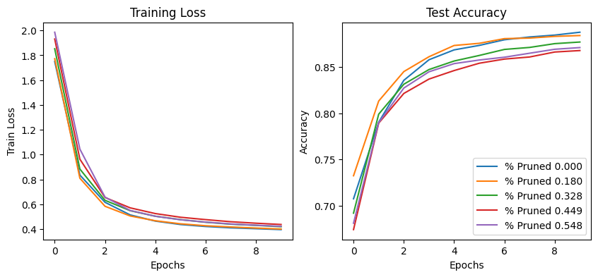
Following the above, we show the different pruning stages of the Intrinsic Dimensionality + Iterative Magnitude Pruning training paradigm. Unsurprisingly, we observe a similar effect to IMP whereby early pruning and reinitialization actually improves performance. However, somewhat shockingly, we see that zeroing out over half of the weights does not have a dramatic effect on model quality. Unlike in the IMP example, the total number of trainable parameters is 256 (equivalent to what was selected for the Intrinsic Dimensionality paradigm). This likely means that there is some amount of essential sparseness that must occur for useful internal model representation. This is surprising! Much like how our human brains rely on sparsity of neuronal activation, it appears that over half of all weights (and therefore computations) for a particular model are unnecessary. This is despite the entirety of the weights being a result of a random projection of a lower dimensional parameter space.

Adversarial Robustness of the Dual Axis
For those of you who’ve read my previous blog on Implicit Neural Neural Representations (INNR) models, you might recall that we attacked our models. Adversarial attacks can provide insights on both the nature of a neural network’s decision boundary and their underlying architecture. For instance, the work of Madry et al explores the problem of model capacity in relation to adversarial robustness.
\(\min_{\theta} \rho(\theta)\) where \(\rho(\theta) = E_{(x, y)}[\max_{\delta \in S} L(\theta, x + \delta, y)]\)
Here, \(\rho\) an optimization function generate a set of parameters \(\theta\) that satisfies, \(S\) denotes a set of allowed perturbations for an adversary, and \(L\) is a loss function. They note that the Fast Gradient Sign Method can be considered a constrained first-order step that aims to maximize the inner function.
Madry et al. claim that the capacity for robustness is linked to the capacity of the model. They found that small models, which may normally be able to learn a task, may not be able to learn with adversarial training. Larger models are often more robust, and the greater the capacity, the more reduced an attack may transfer. This intuitively makes sense: if we consider robustness (in this case, robustness around some \(l_{\infty}\) ball surrounding an input) as a different optimization task, you would naturally assume that you would require a larger model to encode this functionality. Here is where we finally may pose the question: ‘How does pruning and dimensionality affect robustness?’
For this exploration, since we already introduce Madry et al let us apply Projected Gradient Descent as our attack vector. The code for projected gradient descent is shared below. Frankly it is simply a constrained iterative optimization algorithm that clamps the input to a specified size (allowable by \(S\)).
# Generates an adversarial attack using the projected gradient descent method
def attack(model,
           device,
           test_loader,
           criterion,
           epsilon,
           alpha,
           attack_iter,
           clamp_min,
           clamp_max):
    model.eval()
    adversarial_examples = []
    target_labels = []

    for data, target in test_loader:
        data, target = data.to(device), target.to(device)
        data.requires_grad = True

        perturbation = torch.zeros_like(data).uniform_(-epsilon, epsilon)

        for _ in range(attack_iter):
            output = model(data + perturbation)
            loss = criterion(output, target)
            loss.backward()

            with torch.no_grad():
                perturbation += alpha * torch.sign(data.grad)
                perturbation = torch.clamp(perturbation, -epsilon, epsilon)
                perturbed_data = torch.clamp(data + perturbation, clamp_min, clamp_max)

        adversarial_examples.append(perturbed_data.detach())
        target_labels.append(target.detach())

    return torch.concat(adversarial_examples), torch.concat(target_labels)
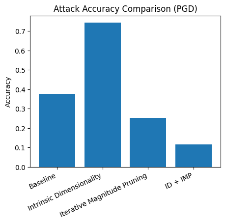
Below, we see some interesting patterns. It appears that pruned networks are uniquely vulnerable to adversarial attacks, even more so than the baseline model from which the attacks were generated. I believe this property to be more related to the nature of pruning than the exact gradient path a model takes (remember for ID + IMP the parameters are randomly projected back atop the initial weights). Relating back to the capacity problem: since pruned networks are in effect small subnetworks (or lottery tickets), their propensity for solving a specific individual task remains high, but their robustness to new tasks remains low. Surprisingly, intrinsic dimensionality remained quite robust to attacks. I hypothesize that this is because the gradient path that was traversed by the parameters was smoother and sufficiently different from the baseline model to offer some protection. As for the gap between the pruned ID variant and the non-pruned variant, I’m not too sure. My best guess is that the pruning of ID pushed the model to follow a similar path to IMP with some number of ‘necessary’ subnetworks being discovered then which were attacked by PGD.

Conclusion
Today, we investigated the interplay between two related but separate concepts: sparsity and dimensionality. We found that we may compress dimensionality further than sparsity to achieve similar performance. We also discover that sparsity does improve performance even if the weights being pruned are the result of a random projection from a shared lower dimensional parameter space. To me, this speaks of a fundamental necessity for network size even if the solution space is found on a lower-dimensional manifold than the total network. This aligns with our intuition behind the manifold hypothesis, suggesting that networks also fall onto a manifold much the same way the data they model do (somewhat unsurprising). Furthermore, we found that given the same initialization but different training schemes, intrinsic dimensionality is surprisingly robust to Projected Gradient Descent attacks, whereas pruned networks are uniquely vulnerable. This poses interesting questions about the nature of how these attacks are generated. A link to the original Google Colab is provided here.