The INNR Monologue
A introduction to Implicit Neural Neural Representation (INNR) models
Introduction
For practitioners of Artificial Intelligence, it is often said that the North Star of our efforts is Artificial General Intelligence (AGI). However, this rather simple goal is itself incredibly ill-defined and nebulous. There exists a large body of work that discusses the topic of the meaning of AGI and what it would mean for a machine to be truly considered intelligent. Today, I offer my own humble perspective on the topic: I believe AGI is achieved when a machine approximates the function of a human being. What do I mean by this?
The beauty of human beings and my fascination with them (and by extension AI) is the diversity and similarity among people. Despite a great and wondrous variety of thought and circumstance, there exists a remarkable amount of overlap and commonality between people that unify the human experience. It appears that for many people, they share in learning many of the same things, resulting in clichés that, while perhaps mundane, remain true for most, if not all, individuals. It is likely that all of us, at some point, will learn through our own experiences what it means to feel pride, joy, hunger, and grief.
Indeed, these patterns, to me, speak of a greater overarching idea: there is some process through which humans must go while on the path to acquiring cognition akin to general intelligence. If we consider an individual human’s consciousness as a datum, it is this process that I believe the field should aim to replicate for machines.
Background
So how can we accomplish this goal? I turn to the recent advancements in deep learning and neural networks. Heavily oversimplifying, the aim of a neural network is to learn a particular data-generating process. By now, I’m sure you’re aware of the common narrative of learning by example, whereby we feed a neural network many examples of a particular task and it learns through convex optimization. So, in the example of an image classifier, we may feed many examples of image-label pairs so that we can approximate the mapping (or model the data-generating process) from image to label. In reality, neural networks can learn any such function (see Universal Approximation Theorem).
HyperNetworks
Learning a mapping from image to label is all well and good, but in my mind, to achieve true AGI, we must answer the question: “What is the data-generating process for cognition?” If we can define such a function, then is it possible to learn it? The answer (unsurprisingly) is yes! Metalearning is a field that aims to address these questions. While there are a variety of different approaches to meta-learning, in this blog post, I aim to focus on one: hypernetworks.
Hypernetworks are neural networks that have been trained to generate the weights (either in full or in part) of other networks. It is distinct from meta-learning algorithms like MAML
Implicit Neural Representations
Switching gears a bit, Implicit Neural Representations (INR) are a class of neural networks that model discrete signals as continuous by learning a representation that maps values directly from coordinate space. For instance, a color image is a discrete signal of \((r, g, b)\) values that is defined by \((x,\ y)\) coordinates. An implicit neural representation for an image is a function \(f(x,\ y\ |\ \theta)\) with a maximum domain of \((height,\ width)\). Notably, the domain is of fixed size with discrete pixel intervals; however, the learned function is continuous.
\[f(x,\ y\ |\ \theta) → (r_{x, y},\ b_{x, y},\ g_{x, y})\]INRs have been used to map a variety of different data modalities, from images to audio to point clouds to 3D scenes. Popular examples of INRs include Neural Radiance Fields (NeRFs)
Implicit Neural Neural Representation (INNR) models
This work aims to explore that question by introducing the concept of Implicit Neural Neural Representations (INNR) Models. To my knowledge, this is the first work that attempts to apply INRs to completely represent a neural network. INNR models are a class of hypernetwork that only encodes for a single neural network. These models can be thought of as attempting to reconstruct the original model ‘signal’ in a lossy way. The idea is that it may be possible to use INNR models to construct larger models. The goals of this work are as follows:
- Identify the feasibility of representing neural network architectures as a continuous signal.
- Explore the feasibility of INNR models as a form of network compression that does not require any training data other than the weights of the model itself.
- Understand how INNR models may be vulnerable to evasion attacks from their original model.
Initial MNIST Model
To begin, we must define an initial model for which we will attempt to compress. For this exploration, we will consider only the perennial toy dataset MNIST. Shown below is a simplified convolutional neural network that is loosely inspired by the LeNet5 architecture.
class MnistExampleNet(nn.Module):
  """
  A simple convolutional network inspired by LeNet5 for MNIST classification

  Parameters:
      c (int): Number of channels in the first convolutional layer.
  """
  def __init__(self, c: int=32):
    super(MnistExampleNet, self).__init__()
    self.conv1 = nn.Conv2d(1, c, kernel_size=5, bias=False)
    self.pool = nn.MaxPool2d(kernel_size=2, stride=2)
    self.conv2 = nn.Conv2d(c, c * 2, kernel_size=5, bias=False)
    self.fc1 = nn.Linear(c * 2 * 4 * 4, 10, bias=False)

  def forward(self, x):
    x = self.pool(F.sigmoid(self.conv1(x)))
    x = self.pool(F.sigmoid(self.conv2(x)))
    x = x.flatten(1)
    x = self.fc1(x)
    return x
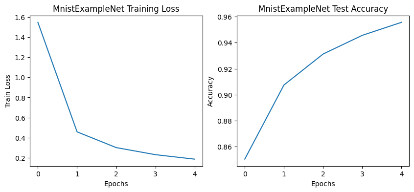
We train this model for only 5 epochs, which is sufficient to achieve adequate convergence for the sake of our testing. The training and accuracy curves of our initial model can be found below.

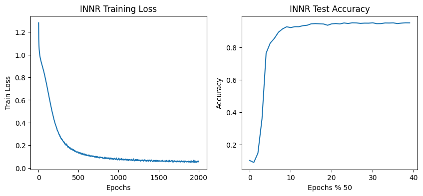
INNR Model Training
We must now decide on a coordinate scheme to train our INNR model. This is challenging as the dimensionality of a network changes depending on the type of layer: convolutional layers have 4 dimensions, linear layers have 2 dimensions, and bias layers have a dimension of 1. The simplest mechanism to map these coordinates is to project the lower-dimensional linear and bias layers as a hyperplane centered around the origin. Note that the domain varies significantly across layers, with \((channel\ out,\ channel\ in,\ filter\ height,\ filter\ width)\) as the domain of convolutional layers, \((output,\ input)\) as the domain of linear layers, and \((output)\) as the domain of bias layers.
Therefore, our coordinate scheme is as follows:
- \((layer,\ c_{out},\ c_{in},\ w,\ h)\) for convolutional layers
- \((layer,\ out,\ in,\ 0,\ 0)\) for linear layers
- \((layer,\ out,\ 0,\ 0,\ 0)\) for bias layers (omitted for simplicity)
Given that the domain is variable across layers, it’s likely that the manifold learned by the INNR model is more intricate compared to models dealing with consistent domains, such as images or audio. We normalize the domain of each dimension of a layer to \([-1,\ 1]\). The code for this dataset can be found below.
class ConvCoordinateDataset(Dataset):
  """
  Dataset class for handling neural network coordinates and weights.

  Args:
    params (Tuple[torch.Tensor]): Tuple of parameter tensors
    standardize (bool): Flag indicating whether to standardize the weights.
  """
  def __init__(self, params: Tuple[torch.Tensor], standardize: bool = True):
    self.weights = self._flatten_params(params)
    self.coordinates = self._convert_to_coordinates(params)
    self.standardize = standardize
    if standardize:
      self.transformed_weights = self.standardize_weights()

  # Flatten the paramneter tuple
  def _flatten_params(self, params: Tuple[torch.Tensor]):
    flat_params = torch.concat([param.cpu().flatten() for param in params])
    return flat_params.view(-1, 1)

  # Translate convolutional params into normalized coordinates (cout, cin, h, w)
  def _conv_coordinates(self, param: torch.Tensor) -> torch.Tensor:
    conv_ranges = [torch.linspace(-1, 1, steps=size) for size in param.shape]
    mgrids = torch.meshgrid(*conv_ranges)
    normalized_coordinates = torch.stack(mgrids, dim=-1).reshape(-1, 4)
    return normalized_coordinates

  # Translate bias params into normalized coordinates (bias, 0, 0, 0)
  def _bias_coordinates(self, param: torch.Tensor) -> torch.Tensor:
    zeroes = torch.zeros(1)
    bias_ranges = torch.linspace(-1, 1, steps=param.shape[0])
    mgrids = torch.meshgrid(bias_ranges, zeroes, zeroes, zeroes)
    normalized_coordinates = torch.stack(mgrids, dim=-1).reshape(-1, 4)
    return normalized_coordinates

  # Translate linear parameters into normalized coordinates (out, in, 0, 0)
  def _lin_coordinates(self, param: torch.Tensor) -> torch.Tensor:
    zeroes = torch.zeros(1)
    lin_ranges = [torch.linspace(-1, 1, steps=size) for size in param.shape]
    mgrids = torch.meshgrid(*lin_ranges, zeroes, zeroes)
    normalized_coordinates = torch.stack(mgrids, dim=-1).reshape(-1, 4)
    return normalized_coordinates

  # Generate Coordinates with range [-1, 1] in form (layer, out, in, h, w)
  def _convert_to_coordinates(self, params: Tuple[torch.Tensor]):
    layer_coords = torch.linspace(-1, 1, steps=len(params))
    coordinates = []
    for param in params:
      if param.ndim == 4:
        coordinates.append(self._conv_coordinates(param))
      if param.ndim == 1:
        coordinates.append(self._bias_coordinates(param))
      if param.ndim == 2:
        coordinates.append(self._lin_coordinates(param))
    for i in range(len(params)):
      layer_coord = torch.full((len(coordinates[i]), 1), layer_coords[i])
      coordinates[i] = torch.concat([coordinates[i], layer_coord], -1)
    return torch.concat(coordinates)

  # Standardize outputs to improve training convergence
  def standardize_weights(self):
    mean, std = self.weights.mean(), self.weights.std()
    standardized_weights = (self.weights - mean) / std
    return standardized_weights

  # Reverse standardization for inference time
  def inverse_standardize_weights(self, weights: torch.Tensor):
    mean, std = self.weights.mean(), self.weights.std()
    standardized_weights = weights * std + mean
    return standardized_weights

  def __len__(self):
    return len(self.coordinates)

  def __getitem__(self, idx):
    weights = self.transformed_weights if self.standardize else self.weights
    return self.coordinates[idx], weights[idx]
The learned INNR model is of the form \(f(l,\ out,\ in,\ x,\ y\ |\ \theta) → \phi_{(l,\ out,\ in,\ x,\ y)}\) where \(\phi\) is the parameter at the given layer coordinates. I use the popular SIREN

Results

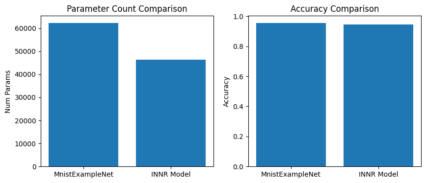
As shown above, we see that the performance of the INNR model’s produced model is comparable to the initial model while having roughly 20% fewer parameters. The difference in performance was expected, as INRs are lossy when encoding their mediums. While other techniques may result in smaller networks of comparable quality, what makes this method notable is the exclusion of any training or testing data. The INNR model fully encoded the initial convolutional neural network. However, since we are directly approximating the target network, it does mean that we also reconstruct the potential vulnerabilities of the initial models as well.
Attacking the INNR model
An adversarial example is a manipulated input data sample that has been perturbed to cause an unexpected outcome. This is typically done by backpropagation through a target network. As our INNR model attempts to approximate the initial network, it too should be vulnerable to any attacks that are generated from the initial network. We test out this hypothesis empirically. For this task, we use the Fast Gradient Sign Method introduced by GoodFellow et al
# Generates an adversarial attack using the fast gradient sign method
def attack(model: nn.Module,
          device: torch.device,
          test_loader: DataLoader,
          criterion: nn.Module,
          epsilon=0.1):
  model = model.to(device)
  model.eval()
  attacks, targets = [], []
  for batch_idx, (data, target) in enumerate(test_loader):
    data, target = data.to(device), target.to(device)
    data.requires_grad = True
    output = model(data)
    loss = criterion(output, target)
    model.zero_grad()
    loss.backward()
    attack = data + epsilon * torch.sign(data.grad.data)
    attacks.append(attack)
    targets.append(target)
  return torch.concat(attacks), torch.concat(targets)
We investigate adversarial attacks to understand the reconstruction error of the INNR model. If the model is faithfully reconstructed then we expect the adversarial attacks to transfer, which we can see in the below figure.

Conclusion
This project was chosen as the code snippet for review for Christopher Wang’s MILA application for Fall of 2024. This project is ideal because of its limited scope, ease of readability, and interesting results. All experiments were conducted on Google Colab using a T4. A link to the the original Google Colab is provided here.